What is Genetic Ancestry?
While so far I have mostly talked about using statistics to identify SNPs associated with a particular trait, this is not the only thing statistical geneticists do. Companies like 23andMe or AncestryDNA profit by selling DNA testing kits and returning the customer with a comprehensive ancestry breakdown. How do they do this?
What genetic ancestry does is look at the ancestral origin of the genetic material we actually inherited. While we often think of being “1/4 Irish” or “1/8 North African”, we don’t actually inherit exactly 1/4 of our grandparents’ genetic material. As DNA is passed from one generation to the next, recombination events happen that shuffle up the genetic material. So while we have the same genealogical ancestry as our siblings, genetic ancestry isn’t the same. We can think of our genetic ancestry in two ways - locally and globally. Local ancestry refers to inheriting a specific part of your genome from an ancestor of a particular category. Global ancestry looks across the whole genome and refers to inheriting a proportion of your genome from an ancestor of a particular category.
There are difficulties to determining someone’s local and global ancestry. It is hard to figure out which ancestor you got each portion of your genome from, and you need good information about which ancestry categories those ancestors belonged to. Due to these challenges, the focus is more on which segments of your genome are similar to individuals from a specific category. There are still challenges with this, which include how to define “similarity”, at what level to define categories (Swedish vs Scandinavian vs European), and finding people from each category to compare your genome to. The two large classes of statistical methods that are used to infer genetic similarity are machine learning tools (including PCA, regression forests, and support vector machines) and model-based, biologically informed approaches (including bayesian methods, maximum likelihood estimation, and others).
The Genetic Ancestry of African Americans, Latinos, and European Americans across the U.S.
To learn more about genetic ancestry, we read a paper in class titled “The Genetic Ancestry of African Americans, Latinos, and European Americans Across the United States” published in 2015 and written by Katarzyna Bryc, Eric Y. Durand, Michael J. Macpherson, David Reich, and Joanna Mountain. This study looks at the genetic ancestry of 5,269 African-Americans, 8,663 Latinos, and 148,789 European Americans who are 23andMe customers and shows that historical interactions between the groups are present in the genetic-ancestry of Americans today (Price et al. 2010). This paper was very dense, but I had a few main takeaways from it.
First, the authors used what they called “Ancestry Composition” which assigns ancestry labels to short local phased genomic regions and produces local ancestry proportions and confidence scores. This method provides ancestry proportions for several worldwide populations at each window the genome. If a window has a majority of a continental ancestry (>51%), that window is counted in the number of windows inherited from the ancestry. So to estimate the proportion of a particular ancestry someone is, you divide the number of windows of that ancestry they have by the total number of windows studied.
The authors also wanted to understand the time frame of admixture events, and to do so they used simple admixture models and grid search optimization. With this method and their ancestry composition method described above, they were able to come up with some interesting results. They were able to find differences in ancestry proportions between slave and free states and learned 1/5 of Africans have Native American ancestry. For the Latino group, they saw high levels of Iberian ancestry appear in areas of high Native American ancestry. Additionally, the noted that European ancestry not homogenous across US, which likely reflects immigration patterns of different ethnic groups.
Genetic Ancestry and its confounding role in GWAS
Genetic ancestry is not only studied to determine whether or not we can see historical interactions present in the genetics of Americans today. Genetic ancestry is also important because it is a potential confounding variable in GWAS. When we are trying to determine if a particular SNP has a relationship with our trait of interest, we have to keep in mind the role of ancestry. Ancestry has a relationship with genotypes because the allele frequency of the SNP we’re testing differs across ancestral populations. Additionally, ancestry can have a relationship with our trait of interest - environmental factors or causal SNPs in other parts of the genome can differ across ancestry groups.
Knowing that genetic ancestry is a confounding variable, we should adjust for it in our GWAS models with the following equation, where \(y\) is the trait, \(x_j\) is the number of minor alleles at position \(j\), and \(\pi\) is the genetic ancestry.
\[E[y|x_j, \pi] = \alpha + \beta_j x_j + \gamma\pi \\\]
Before completing the GWAS, we will need to infer genetic ancestry using one of the methods mentioned earlier. Here we will use PCA.
PCA background
Principal component analysis (PCA) is a widely used technique for dimension reduction. Dimension reduction aims to represent the information within our data with fewer variables, which is perfect for genetic data where we have millions of SNPs. With PCA, we are specifically looking for linear transformation of our data that explains the most variability. This linear representation is composed of principal components, or PCs. These PCs are new variables that are a linear combinations of our original SNPs:
\[PC_1 = a_{11}x_1 + a_{12}x_2 + \cdots + a_{1p}x_p\] \[PC_2 = a_{21}x_1 + a_{22}x_2 + \cdots + a_{2p}x_p\] \[....\] \[PC_p = a_{p1}x_1 + a_{p2}x_2 + \cdots + a_{pp}x_p\]
The number of the PC has some meaning to it - \(PC_1\) is the component that explains the most variability in our data when all possible linear combinations are considered. In other words, it has the highest variance. \(PC_2\) has the next highest variance, subject to the constraint of being orthogonal to, or uncorrelated with, \(PC_1\). Next is \(PC_3\), which is orthogonal to \(PC_2\), and so forth.
Other important terminology related to PCs are scores and loadings. Loadings are the coefficients \(a_{11}, a_{22}\), etc, which represent the contribution of each of the original variables to the new PC. Scores are the values that PCs take when you multiply the loading \(a_{pp}\) by the value at that SNP, \(x_p\).
Running PCA on our data
To learn how to run PCA on our dataset, I largely followed this tutorial by Xiuwen Zheng from the Department of Biostatistics at the University of Washington – Seattle (Zheng, n.d.).
Start by loading necessary libraries. If you have trouble installing the SNPRelate package, make sure you follow how to do it exactly as shown in the tutorial.
The next step is to load the data, convert it to GDS format, and combine files. Once you do this once, it will create files on your computer and you do not have to run this code again.
bed.fn.m <- "/Users/erinfranke/Desktop/GWAStutorial-master/public/Genomics/108Malay_2527458snps.bed"
fam.fn.m <- "/Users/erinfranke/Desktop/GWAStutorial-master/public/Genomics/108Malay_2527458snps.fam"
bim.fn.m <- "/Users/erinfranke/Desktop/GWAStutorial-master/public/Genomics/108Malay_2527458snps.bim"

snpgdsBED2GDS(bed.fn.m, fam.fn.m, bim.fn.m, "test.gds")

bed.fn.i <- "/Users/erinfranke/Desktop/GWAStutorial-master/public/Genomics/105Indian_2527458snps.bed"
fam.fn.i <- "/Users/erinfranke/Desktop/GWAStutorial-master/public/Genomics/105Indian_2527458snps.fam"
bim.fn.i <- "/Users/erinfranke/Desktop/GWAStutorial-master/public/Genomics/105Indian_2527458snps.bim"

snpgdsBED2GDS(bed.fn.i, fam.fn.i, bim.fn.i, "test2.gds")

bed.fn.c <- "/Users/erinfranke/Desktop/GWAStutorial-master/public/Genomics/110Chinese_2527458snps.bed"
fam.fn.c <- "/Users/erinfranke/Desktop/GWAStutorial-master/public/Genomics/110Chinese_2527458snps.fam"
bim.fn.c <- "/Users/erinfranke/Desktop/GWAStutorial-master/public/Genomics/110Chinese_2527458snps.bim"

snpgdsBED2GDS(bed.fn.c, fam.fn.c, bim.fn.c, "test3.gds")

snpgdsSummary("test.gds")

fn1 <- "test.gds"
fn2 <- "test2.gds"
fn3 <- "test3.gds"
snpgdsCombineGeno(c(fn1, fn2, fn3), "test4.gds")
Next, get a summary of the combined file and open it.
snpgdsSummary("test4.gds")The file name: /Users/erinfranke/Desktop/MACStats/Statistical Genetics/finalcontentsummary/test4.gds
The total number of samples: 323
The total number of SNPs: 2176501
SNP genotypes are stored in SNP-major mode (Sample X SNP).
The number of valid samples: 323
The number of biallelic unique SNPs: 1300388 genofile <- snpgdsOpen("test4.gds")Earlier in the multiple testing section I talked a little bit about correlation between SNPs and linkage disequilibrium. When doing PCA, its suggested to use a pruned set of SNPs which are in approximate linkage equilibrium with each other to avoid the strong influence of SNP clusters. The following code tries different LD thresholds and selects a set of SNPs.
set.seed(1000)

# Try different LD thresholds for sensitivity analysis
snpset <- snpgdsLDpruning(genofile, ld.threshold=0.2)
SNP pruning based on LD:
Excluding 0 SNP on non-autosomes
Excluding 876,113 SNPs (monomorphic: TRUE, MAF: NaN, missing rate: NaN)
# of samples: 323
# of SNPs: 1,300,388
using 1 thread
sliding window: 500,000 basepairs, Inf SNPs
|LD| threshold: 0.2
method: composite
Chromosome 1: 4.54%, 8,114/178,671
Chromosome 2: 4.27%, 7,658/179,463
Chromosome 3: 4.58%, 6,933/151,523
Chromosome 4: 4.55%, 6,304/138,560
Chromosome 5: 4.54%, 6,051/133,424
Chromosome 6: 4.13%, 5,916/143,125
Chromosome 7: 4.59%, 5,473/119,147
Chromosome 8: 4.33%, 4,954/114,456
Chromosome 9: 4.76%, 4,637/97,371
Chromosome 10: 4.68%, 5,109/109,218
Chromosome 11: 4.20%, 4,718/112,258
Chromosome 12: 4.70%, 5,024/106,902
Chromosome 13: 5.03%, 3,724/74,013
Chromosome 14: 4.85%, 3,499/72,089
Chromosome 15: 4.97%, 3,445/69,297
Chromosome 16: 4.97%, 3,717/74,739
Chromosome 17: 5.13%, 3,515/68,572
Chromosome 18: 5.54%, 3,443/62,121
Chromosome 19: 4.99%, 2,713/54,393
Chromosome 20: 5.30%, 2,841/53,560
Chromosome 21: 5.32%, 1,613/30,341
Chromosome 22: 5.25%, 1,747/33,258
101,148 markers are selected in total.str(snpset)List of 22
$ chr1 : chr [1:8114] "rs11240777" "kgp9059038" "rs7537756" "exm628" ...
$ chr2 : chr [1:7658] "kgp4971557" "kgp14800530" "rs17041717" "kgp2057000" ...
$ chr3 : chr [1:6933] "kgp7646170" "kgp3611083" "kgp4281785" "kgp5157934" ...
$ chr4 : chr [1:6304] "kgp7767085" "kgp7706308" "kgp10870542" "rs6847267" ...
$ chr5 : chr [1:6051] "kgp2306997" "kgp9525211" "kgp7091813" "kgp10311375" ...
$ chr6 : chr [1:5916] "kgp22745386" "kgp22734311" "kgp22752232" "kgp22744524" ...
$ chr7 : chr [1:5473] "kgp3293955" "kgp2819807" "kgp4314509" "kgp6561807" ...
$ chr8 : chr [1:4954] "kgp8876035" "kgp5401210" "kgp12018201" "kgp1622190" ...
$ chr9 : chr [1:4637] "rs680654" "kgp3928777" "kgp3538210" "kgp4962798" ...
$ chr10: chr [1:5109] "kgp10879287" "rs3125037" "kgp22052249" "kgp21937175" ...
$ chr11: chr [1:4718] "exm869284" "rs2272566" "kgp6770543" "kgp9403358" ...
$ chr12: chr [1:5024] "kgp8962939" "rs1106984" "rs7135126" "rs7974784" ...
$ chr13: chr [1:3724] "kgp6812842" "kgp1456930" "kgp200360" "rs9580112" ...
$ chr14: chr [1:3499] "kgp3297105" "exm1083420" "Exome_Asian_chr14-20296278-19" "kgp11118585" ...
$ chr15: chr [1:3445] "kgp1349873" "rs4932072" "kgp6048141" "Exome_Asian_chr15-20588685-19" ...
$ chr16: chr [1:3717] "kgp4996586" "kgp11473370" "kgp571139" "kgp9353104" ...
$ chr17: chr [1:3515] "kgp9690030" "kgp942802" "kgp7899711" "rs7223759" ...
$ chr18: chr [1:3443] "rs8096369" "kgp27746" "rs621636" "kgp5913270" ...
$ chr19: chr [1:2713] "kgp21362931" "kgp4747527" "kgp574339" "kgp12372026" ...
$ chr20: chr [1:2841] "rs6139074" "rs6039403" "kgp8039653" "kgp10171668" ...
$ chr21: chr [1:1613] "rs12627229" "exm1562172" "kgp13170864" "kgp11190641" ...
$ chr22: chr [1:1747] "kgp1568720" "rs5747010" "kgp8641560" "rs16980739" ...names(snpset) [1] "chr1" "chr2" "chr3" "chr4" "chr5" "chr6" "chr7" "chr8"
[9] "chr9" "chr10" "chr11" "chr12" "chr13" "chr14" "chr15" "chr16"
[17] "chr17" "chr18" "chr19" "chr20" "chr21" "chr22"[1] "rs11240777" "kgp9059038" "rs7537756" "exm628" "rs1891910"
[6] "kgp7634233"We can then run PCA and calculate the percent of variation is accounted for by the top principal components. It looks like the first principal component explains 3.13% of variation, the second explains 0.85%, the third and fourth explain 0.43%, the fifth 0.39%, etc. Therefore, the optimal number of principal components to use is probably 2.
# Run PCA
pca <- snpgdsPCA(genofile, snp.id=snpset.id, num.thread=2)
Principal Component Analysis (PCA) on genotypes:
Excluding 2,075,353 SNPs (non-autosomes or non-selection)
Excluding 0 SNP (monomorphic: TRUE, MAF: NaN, missing rate: NaN)
# of samples: 323
# of SNPs: 101,148
using 2 threads
# of principal components: 32
PCA: the sum of all selected genotypes (0,1,2) = 10950024
CPU capabilities: Double-Precision SSE2
Sat Dec 10 18:12:13 2022 (internal increment: 1508)
[..................................................] 0%, ETC: ---
[==================================================] 100%, completed, 2s
Sat Dec 10 18:12:15 2022 Begin (eigenvalues and eigenvectors)
Sat Dec 10 18:12:15 2022 Done. [1] 3.13 0.85 0.43 0.43 0.39 0.38 0.38 0.37 0.37 0.37 0.37 0.37 0.36
[14] 0.36 0.36 0.36 0.36 0.36 0.36 0.36If we didn’t have any prior population information, we could plot the first two principal components and see if we see any patterns in the data. It kind of looks like we have three separate populations, which we know to be true!
# make a data.frame
tab <- data.frame(sample.id = pca$sample.id,
    EV1 = pca$eigenvect[,1],    # the first eigenvector
    EV2 = pca$eigenvect[,2],    # the second eigenvector
    stringsAsFactors = FALSE)

# Draw
plot(tab$EV2, tab$EV1, xlab="eigenvector 2", ylab="eigenvector 1")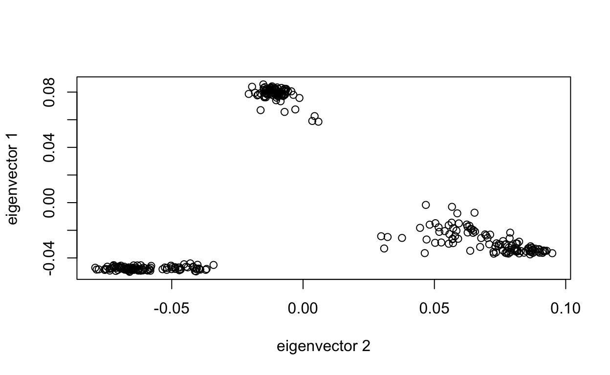
To incorporate prior population, first load the data:
load("/Users/erinfranke/Desktop/GWAStutorial-master/conversionTable.RData")

pathM <- paste("/Users/erinfranke/Desktop/GWAStutorial-master/public/Genomics/108Malay_2527458snps",
               c(".bed", ".bim", ".fam"), sep = "")
SNP_M <- read.plink(pathM[1], pathM[2], pathM[3])

pathI <- paste("/Users/erinfranke/Desktop/GWAStutorial-master/public/Genomics/105Indian_2527458snps",
               c(".bed", ".bim", ".fam"), sep = "")
SNP_I <- read.plink(pathI[1], pathI[2], pathI[3])

pathC <- paste("/Users/erinfranke/Desktop/GWAStutorial-master/public/Genomics/110Chinese_2527458snps",
               c(".bed", ".bim", ".fam"), sep = "")
SNP_C <- read.plink(pathC[1], pathC[2], pathC[3])
Then, run the following code. We can see the three clusters align with the three subpopulations as we expected.
SNP_fam <- rbind(SNP_M$fam, SNP_I$fam, SNP_C$fam) %>%
  mutate(pop = c(rep("Malay", 108), rep("Indian", 105), rep("Chinese", 110)))

sample.id =  SNP_fam$pedigree


tab <- data.frame(sample.id = SNP_fam$pedigree,
    pop = factor(SNP_fam$pop)[match(pca$sample.id, sample.id)],
    EV1 = pca$eigenvect[,1],    # the first eigenvector
    EV2 = pca$eigenvect[,2],    # the second eigenvector
    stringsAsFactors = FALSE)
head(tab)
sample.id pop EV1 EV2
1 M11062205 Malay -0.03507693 0.08154056
2 M11050406 Malay -0.03538905 0.09150315
3 M11050407 Malay -0.03566775 0.08688487
4 M11070602 Malay -0.03317120 0.08035539
5 M11060912 Malay -0.01784295 0.05161642
6 M11060920 Malay -0.02643969 0.05688225plot(tab$EV2, tab$EV1, col=as.integer(tab$pop), xlab="eigenvector 2", ylab="eigenvector 1")
legend("bottomright", legend=levels(tab$pop), pch="o", col=1:nlevels(tab$pop))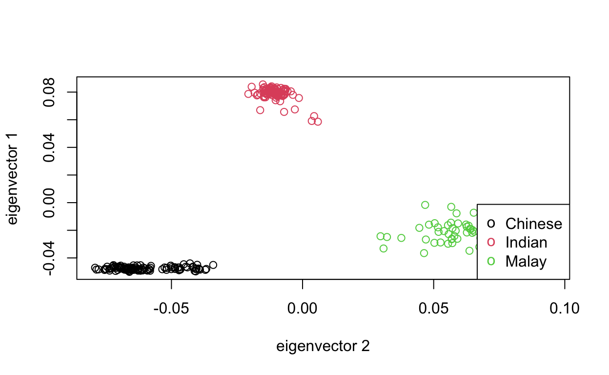
If we wanted to, we could look at the top 4 PCs with the following code and decide whether or not it is worth including PCs 3 & 4 when accounting for genetic ancestry in GWAS. To me, it looks like the clusters overlap a lot less (meaning more variation is explained) when looking at PCs 1 & 2 and PCs 3 & 4 don’t tell us that much (for example, all the dots are on top of each other for the plot of PC3 versus PC4).
lbls <- paste("PC", 1:4, "\n", format(pc.percent[1:4], digits=2), "%", sep="")
pairs(pca$eigenvect[,1:4], col=tab$pop, labels=lbls)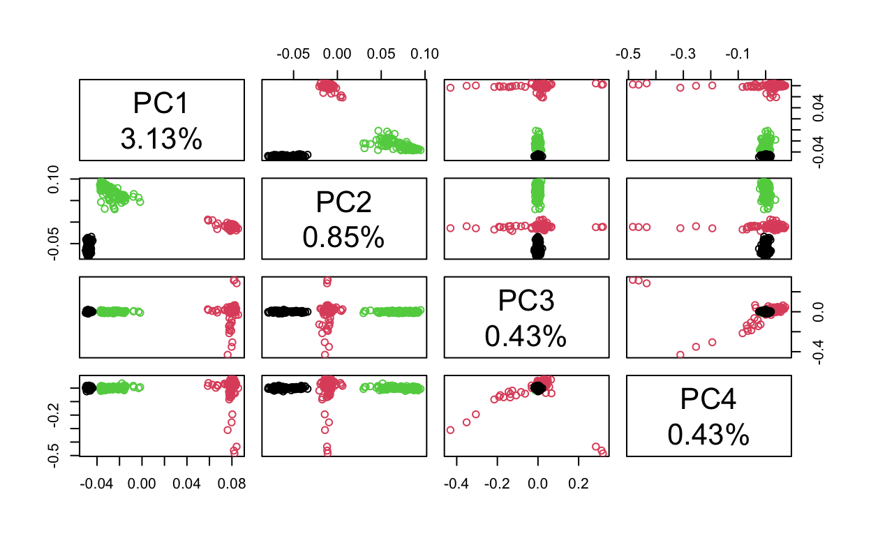
We can also see this in a parallel coordinates plot for the top 16 principal components - starting at PC3 the green sub population (Malay) is completely covered by the red and black lines (Chinese and Indian). This indicates any PCs beyond 1 & 2 are really not helpful significantly to explain variation.
library(MASS)

datapop <- factor(SNP_fam$pop)[match(pca$sample.id, sample.id)]
parcoord(pca$eigenvect[,1:16], col = datapop)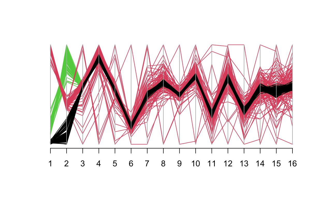
Incorporating PCA into GWAS
Having completed PCA, we can now incorporate PC1 and PC2 into our GWAS. This allows us to adjust for the confounding role that ancestry plays in identifying relationships between SNPs and the trait of interest.This is important because if I were to create a trait that is correlated with both population and a particular SNP, we would expect the p-value for that particular SNP to be significant and easily identifiable. However, when we don’t include the top PCs in our marginal regression models we may get additional SNPs that have significant p-values, specifically SNPs that differ the most in minor allele frequency between the three groups. Including PC1 and PC2 will better account for these ancestral differences and reduce the probability of spurious associations (2+ variables are associated but not causally related due to an unseen factor).
The first step to including principal components in our GWAS is to again convert the SnpMatrix to numeric and generate a trait based on the causal SNP.
I then took the member and pedigree columns on the 323 individuals and created a trait varying based on sub population. After that, I added the trait based on the causal SNP rs3131972 to the trait varying based on sub population to create a trait that varies based on sub population AND one SNP. I sent this file to where the data is stored.
set.seed(494)
rbloggers_popSNP <- cbind(rbloggers_fam %>% dplyr::select(1:2),
                          trait = c(rnorm(n = 108, mean = 0, sd = 1), rnorm(105, -1, sd = 1), rnorm(110, 1, 1)), y) %>%
  mutate(trait = trait + y)

write_delim(rbloggers_popSNP,
            "/Users/erinfranke/Desktop/MACStats/Statistical Genetics/StatGenWillErin/rbloggersSep/rbloggers_popSNP")
To learn how to incorporate principal components in PLINK, I found this set of exercises from Tufts University.
I started by running a GWAS in PLINK without PCs using the code ./plink --bfile rbloggersComb --assoc --pheno rbloggers_popSNP --maf 0.05 --out gwasNoPCA. Next, I read the results into RStudio and created a QQ plot and got a lambda value. This lambda represents the genomic control (GC), which measures the extent of inflation of association based test statistics due to population stratification or other confounders. A value of \(\lambda_{GC} \approx 1\) indicates no stratification, while typically \(\lambda_{GC} > 1.05\) indicates stratification or other confounders including family structure, cryptic relatedness, or differential bias (spurious differences in allele frequencies between cases and controls due to differences in sample collection, sample preparation, and/or genotyping assay procedures). With a \(\lambda_{GC}\) of 1.73 and the QQ plot not fitting the expected distribution, its clear that there is stratification in this data and our p-values are inflated. Hopefully PCA can help account for this.
results_noPCA <- read_table(
  "/Users/erinfranke/Desktop/MACStats/Statistical Genetics/StatGenWillErin/rbloggersSep/gwasNoPCA.qassoc") %>%
  arrange(P)

head(results_noPCA)
# A tibble: 6 × 10
CHR SNP BP NMISS BETA SE R2 T P X10
<dbl> <chr> <dbl> <dbl> <dbl> <dbl> <dbl> <dbl> <dbl> <lgl>
1 2 rs13403822 1.73e8 323 1.32 0.200 0.119 6.58 1.97e-10 NA
2 2 kgp779520 1.73e8 323 1.28 0.202 0.112 6.36 7.14e-10 NA
3 2 kgp5773487 1.10e8 322 1.56 0.247 0.111 6.32 8.95e-10 NA
4 2 rs12624292 1.73e8 323 1.26 0.202 0.108 6.23 1.49e- 9 NA
5 2 rs11892858 1.73e8 323 1.22 0.200 0.104 6.12 2.75e- 9 NA
6 13 kgp4920926 2.62e7 323 -1.34 0.223 0.101 -6.01 5.15e- 9 NA 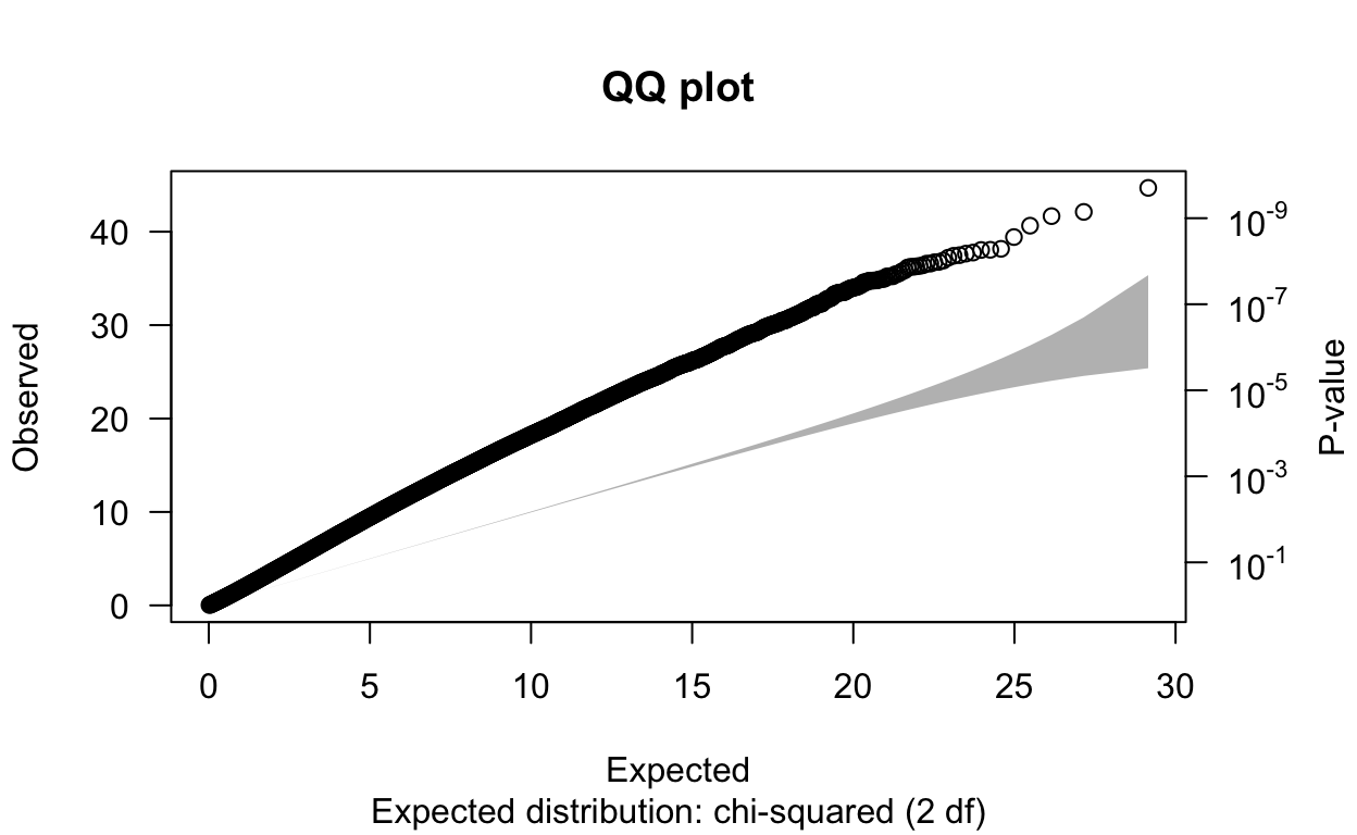
           N      omitted       lambda
1.200898e+06 0.000000e+00 1.731327e+00
To run a GWAS with PCs, I created a pcs.txt file that includes member, pedigree, pc1, and pc2 with the following code and stored it with the rest of my data. To learn how to structure that file correctly, I looked at these slides from Colorado University.
           pedigree    member         pc1        pc2
M11062205 M11062205 M11062205 -0.03507693 0.08154056
M11050406 M11050406 M11050406 -0.03538905 0.09150315
M11050407 M11050407 M11050407 -0.03566775 0.08688487
M11070602 M11070602 M11070602 -0.03317120 0.08035539
M11060912 M11060912 M11060912 -0.01784295 0.05161642
M11060920 M11060920 M11060920 -0.02643969 0.05688225write_delim(pcs, "/Users/erinfranke/Desktop/MACStats/Statistical Genetics/StatGenWillErin/rbloggersSep/pcs")Then, I ran ./plink --bfile rbloggersComb --assoc --covar pcs.txt --covar-name pc1, pc2 --pheno rbloggers_popSNP --out gwasPCA in PLINK and read the results into RStudio below. We can see that the \(\lambda_{GC}\) value went down from 1.73 to 1.61. This means that genetic ancestry did have some kind of confounding effect on the relationship between the SNPs and our trait of interest, so it is good we included them.
results_PCA <- read_table(
  "/Users/erinfranke/Desktop/MACStats/Statistical Genetics/StatGenWillErin/rbloggersSep/gwasPCA.qassoc") %>%
  arrange(P)
head(results_PCA)
# A tibble: 6 × 10
CHR SNP BP NMISS BETA SE R2 T P X10
<dbl> <chr> <dbl> <dbl> <dbl> <dbl> <dbl> <dbl> <dbl> <lgl>
1 2 rs13403822 1.73e8 323 1.32 0.200 0.119 6.58 1.97e-10 NA
2 2 kgp779520 1.73e8 323 1.28 0.202 0.112 6.36 7.14e-10 NA
3 2 kgp5773487 1.10e8 322 1.56 0.247 0.111 6.32 8.95e-10 NA
4 2 rs12624292 1.73e8 323 1.26 0.202 0.108 6.23 1.49e- 9 NA
5 2 rs11892858 1.73e8 323 1.22 0.200 0.104 6.12 2.75e- 9 NA
6 13 kgp4920926 2.62e7 323 -1.34 0.223 0.101 -6.01 5.15e- 9 NA 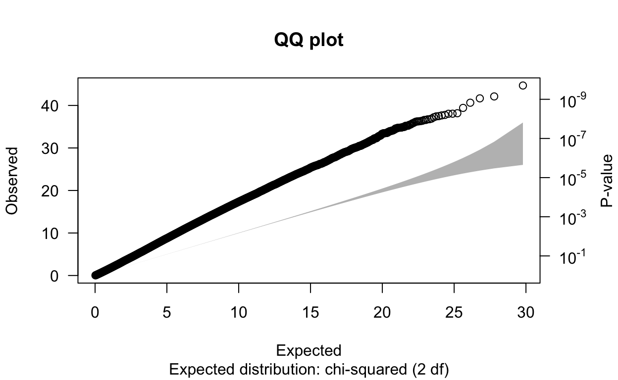
           N      omitted       lambda
1.651345e+06 0.000000e+00 1.613123e+00
One method to correct for inflated \(\lambda_{GC}\) values is to divide association statistics by \(\lambda_{GC}\). This usually provides a sufficient correction for stratification in the case of genetic drift, meaning random fluctuations in allele frequencies over time due to sampling effects, particularly in small populations. However, in the case of ancient population divergence (when populations accumulate independent genetic mutations overtime time and become more different), dividing by \(\lambda_{GC}\) is unlikely to be adequate because SNPs with unusual allele frequency differences that lie outside the expected distribution could be this way because of natural selection. Therefore, there need to be additional approaches to accounting for population stratification than just dividing association statistics by \(\lambda_{GC}\). These approaches include PCA, but also family based association tests and perhaps most effectively mixed models with PC covariates. I think mixed models with PC covariates would really help lower the \(\lambda_{GC}\) value of this dataset as that proved the most effective method for accounting for population stratification in the paper, “New approaches to population stratification in genome-wide association studies” (Price et al. 2010). I don’t know quite how to do this for genetic data yet but I am looking forward to learning more in the future!