Throughout this site, I will go through examples of how to perform statistical techniques to better understand genetic data. To do this, I will rely on a publicly available dataset I downloaded from R-bloggers (Lima 2017), which includes 323 individuals (110 Chinese, 105 Indian and 108 Malay) and 2,527,458 SNPs.
Data Loading and Organization
The following code chunks outline the steps of importing the genetic data.
Load libraries:
Load data for the Chinese, Indian, and Malay individuals and combine them into one SnpMatrix. This process uses read.plink(), which reads a genotype matrix, information on the study’s individuals, and information on the SNPs.
load("GWAStutorial-master/conversionTable.RData")

pathM <- paste("GWAStutorial-master/public/Genomics/108Malay_2527458snps", c(".bed", ".bim", ".fam"), sep = "")
SNP_M <- read.plink(pathM[1], pathM[2], pathM[3])

pathI <- paste("GWAStutorial-master/public/Genomics/105Indian_2527458snps", c(".bed", ".bim", ".fam"), sep = "")
SNP_I <- read.plink(pathI[1], pathI[2], pathI[3])

pathC <- paste("GWAStutorial-master/public/Genomics/110Chinese_2527458snps", c(".bed", ".bim", ".fam"), sep = "")
SNP_C <- read.plink(pathC[1], pathC[2], pathC[3])

SNP <- rbind(SNP_M$genotypes, SNP_I$genotypes, SNP_C$genotypes)
Execute additional data preparation steps recommended by R-bloggers site.
# Take one bim map (all 3 maps are based on the same ordered set of SNPs)
map <- SNP_M$map
colnames(map) <- c("chromosome", "snp.name", "cM", "position", "allele.1", "allele.2")

# Rename SNPs present in the conversion table into rs IDs
mappedSNPs <- intersect(map$SNP, names(conversionTable))
newIDs <- conversionTable[match(map$SNP[map$SNP %in% mappedSNPs], names(conversionTable))]
map$SNP[rownames(map) %in% mappedSNPs] <- newIDs
Exploratory Data Analysis
First, get information about the genotype data. As stated earlier, we have 323 individuals and 2,527,458 SNPs.
SNPA SnpMatrix with 323 rows and 2527458 columns
Row names: M11062205 ... M11082406
Col names: rs4477212 ... kgp22743944 Next, look at the information we have on the individuals in the study. Theoretically, this gives information on family relationships with pedigree, father, and mother, but the father and mother variables contain only missing values. We also have information on the individual’s binary sex, with 1 representing male and 2 female. The affected column represents if the individual had the trait of interest or not, but we are not given that information in this data set so we will simulate a trait later in this analysis.
           pedigree    member father mother sex affected
M11062205 M11062205 M11062205     NA     NA   2       NA
M11050406 M11050406 M11050406     NA     NA   1       NA
M11050407 M11050407 M11050407     NA     NA   1       NA
M11070602 M11070602 M11070602     NA     NA   2       NA
M11060912 M11060912 M11060912     NA     NA   2       NA
M11060920 M11060920 M11060920     NA     NA   2       NA
Finally, we can look at the information we have on each SNP. This tells us a few things:
chromosomeis the number chromosome (typically 1-23) that the SNP is located on.
1is the largest chromosome (most SNPs) and chromosome size typically decreases from there.
snp.nameis the name of the SNP
cMstands for centiMorgans, which is a unit for genetic distance. It represents an estimate of how far SNPs are from one another along the genome.
positiontells us the base pair position of the SNP, with position being being the first nucleotide in our DNA sequence.
- This number restarts from 1 at each chromosome.
- This number restarts from 1 at each chromosome.
allele.1is one of the alleles at this SNP, here the minor allele.
allele.2is the other allele at this SNP, here the major allele.
head(map) chromosome snp.name cM position allele.1 allele.2
rs4477212 1 rs4477212 NA 82154 <NA> A
kgp15717912 1 kgp15717912 NA 534247 <NA> C
kgp7727307 1 kgp7727307 NA 569624 <NA> C
kgp15297216 1 kgp15297216 NA 723918 <NA> G
rs3094315 1 rs3094315 NA 752566 G A
rs3131972 1 rs3131972 NA 752721 A GData Cleaning
One useful piece of information not contained in the data is the minor allele frequency (MAF). This represents the frequency of the minor allele in the dataset. We can add this to our SNP information using the snpstats package and add MAF to map, our data frame that gives us SNP information.
#calculate MAF
maf <- col.summary(SNP)$MAF

# add new MAF variable to map
map <- map %>%
  mutate(MAF = maf)
head(map)
chromosome snp.name cM position allele.1 allele.2
rs4477212 1 rs4477212 NA 82154 <NA> A
kgp15717912 1 kgp15717912 NA 534247 <NA> C
kgp7727307 1 kgp7727307 NA 569624 <NA> C
kgp15297216 1 kgp15297216 NA 723918 <NA> G
rs3094315 1 rs3094315 NA 752566 G A
rs3131972 1 rs3131972 NA 752721 A G
MAF
rs4477212 0.000000000
kgp15717912 0.000000000
kgp7727307 0.001572327
kgp15297216 0.000000000
rs3094315 0.139318885
rs3131972 0.233746130Just looking at the MAF for the first six SNPs in our data, we see that in some cases the minor allele frequency is 0. This means that the SNP is monomorphic - everyone in the dataset has the same genotype at these positions. We will remove these monomorphic SNPs - if everyone has the same alleles at a SNP, there is no variation and we cannot find an association between the minor allele and the trait.
It can also help to think about why we remove SNPs with a MAF of 0 in a mathematical way. If we are trying to fit a line between the trait of interest and SNP 1, we could model this in the following formats, with linear regression listed first and matrix notation second.
\[E[Y|\text{SNP1}] = \beta_0 + \beta1 \text{SNP1}\] \[E[\bf{y}|\bf{X}] = \boldsymbol{\beta} X\]
Further exploring the matrix format, it would look like this: \[X\boldsymbol{\beta} = \begin{bmatrix} 1 & 0 \\ 1 & 0 \\ . & . \\ . & . \\ \end{bmatrix} \begin{bmatrix} \beta_0\\ \beta_1 \\ \end{bmatrix}\]
This problematic because we have linear dependence. You can get the column of minor allele counts by multiplying the intercept column by 0 - in other words, the minor allele count column is a linear combination of the intercept column. This makes our design matrix not be full rank, making \(X^TX\) not invertible and the least squares estimator not defined.
Given all these reasons, we remove SNPs with a MAF of 0 using the code below.
After filtering, we have 1,651,345 SNPs remaining. Therefore, we removed 876,113 SNPs.
However, we are not done cleaning the data. Below, when looking at the first six rows of map, we see two NA values for allele.1. In these rows, the minor allele frequency is not quite 0, but it is very small. In fact, in the first row of this data frame the MAF is 1/646, or 0.00157. This represents that out of the 646 alleles studied (2 alleles for each of the 323 people in the data), there was only one minor allele. On SNP 4 in the data, there were only 3 minor alleles (3/646 = 0.00465).
head(map) chromosome snp.name cM position allele.1 allele.2
kgp7727307 1 kgp7727307 NA 569624 <NA> C
rs3094315 1 rs3094315 NA 752566 G A
rs3131972 1 rs3131972 NA 752721 A G
kgp6703048 1 kgp6703048 NA 754063 T G
kgp15557302 1 kgp15557302 NA 757691 <NA> T
kgp12112772 1 kgp12112772 NA 759036 A G
MAF
kgp7727307 0.001572327
rs3094315 0.139318885
rs3131972 0.233746130
kgp6703048 0.027950311
kgp15557302 0.004658385
kgp12112772 0.026397516Why did the study put NA values instead of the one minor allele found? Perhaps they are worried of a machine reading error given that the minor allele was detected only a couple of times, or maybe there was another reason. To better understand these missing values, I created the density plots below.
map %>%
  mutate(missing = as.factor(case_when(is.na(allele.1) ~ "Allele 1 missing",
                             TRUE ~ "Allele 1 Recorded"))) %>%
  ggplot(aes(x=MAF))+
  geom_density(alpha = 0.5, fill = "cadetblue3")+
  theme_classic()+
  facet_wrap(~missing, scales = "free")+
  labs(x = "Minor allele frequency", y = "density")+
  theme(axis.title = element_text(family = "mono"),
        strip.background = element_blank(),
        strip.text = element_text(family = "mono"))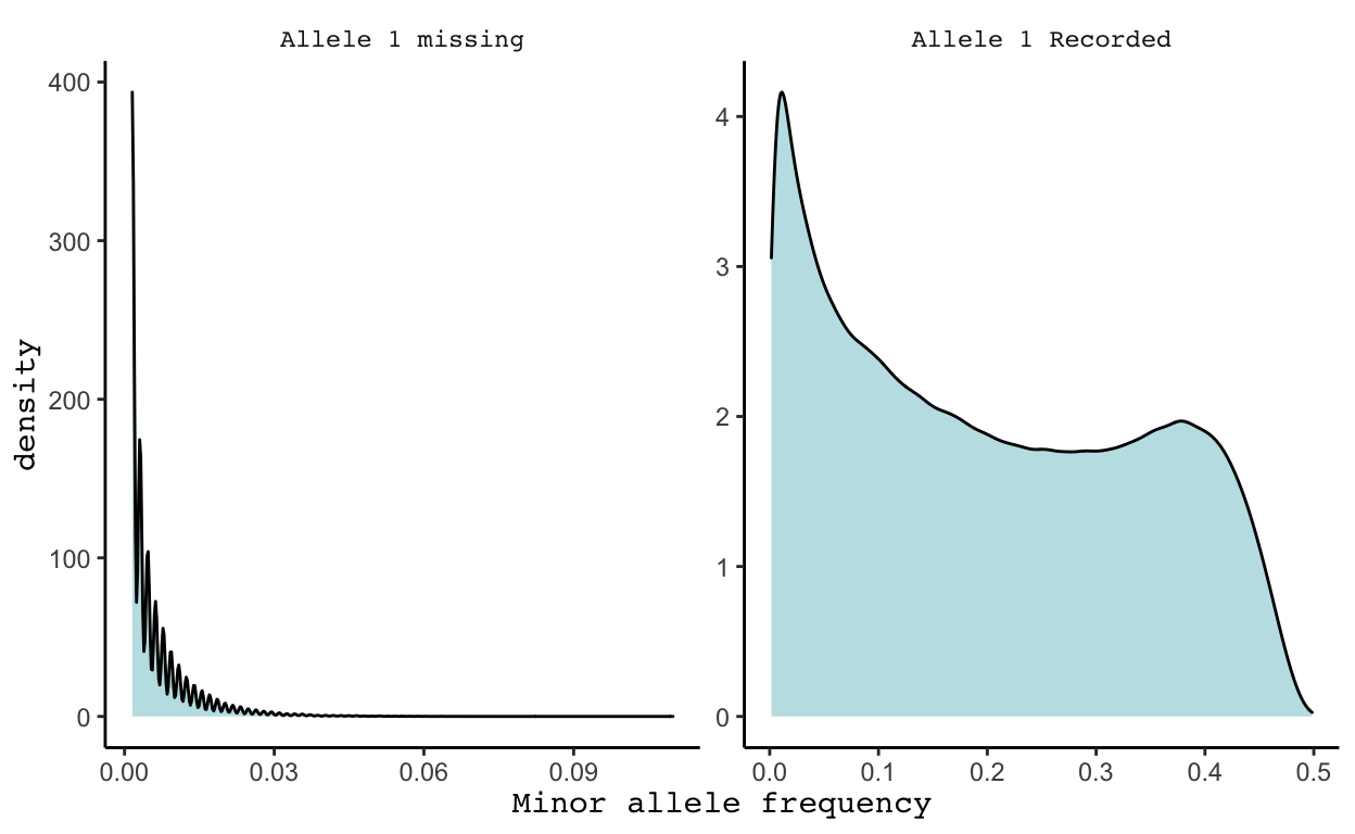
These plots really surprised me. Initially my plan was just to remove all SNPs with a MAF < 1%, figuring that would filter out all SNPs with an NA value for allele 1. However, in the plot above on the left we see that while the majority of allele 1 missing SNPs have a MAF < 1%, some have a MAF close to 11%, meaning about 71/646 minor alleles were detected yet an NA value was still recorded. While I have a very minimal understanding of gene reading machinery, I would not guess that this NA is not a machine reading error but rather that something else is going on. Given this information, I decided to compromise and remove all SNPs with a MAF < 3%, as well as all other SNPs with an NA value for allele 1. This brings us from 1,651,345 SNPs to 1,293,100 SNPs.
One downside to this whole process of removing SNPs with small MAFs is that a major goal of GWAS studies is detect to rare variations on SNPs that could be associated with the trait of interest. Removing SNPs where the MAF is small may result in removing critical data to the study. This is trade off emphasizes that having more people in your GWAS is helpful and important in forming meaningful results about potentially rare variants.
Before moving on, we must complete one final data cleaning step. The snpstats package uses a format in which genotypes are coded as 01, 02, and 03, with 00 representing missing values.
SNP@.Data[1:5,1:5] rs4477212 kgp15717912 kgp7727307 kgp15297216 rs3094315
M11062205 03 03 03 03 03
M11050406 03 03 03 03 03
M11050407 03 03 03 03 03
M11070602 03 03 03 03 02
M11060912 03 03 03 03 03We will convert this to a 0, 1, and 2 format. Now the matrix represents the number of major alleles each person has at each SNP.
X <- as(SNP, "numeric")
X[1:5, 1:5]
rs4477212 kgp15717912 kgp7727307 kgp15297216 rs3094315
M11062205 2 2 2 2 2
M11050406 2 2 2 2 2
M11050407 2 2 2 2 2
M11070602 2 2 2 2 1
M11060912 2 2 2 2 2We also must remove the SNPs with a MAF < 3% and those missing allele 1 from our genotypic matrix X.
Trait Simulation
As discussed earlier, the affected column in our individuals dataset is completely missing values. Therefore, for the purposes of demonstrating how to conduct a GWAS, we will simulate a trait using a random SNP of interest. I randomly chose SNP rs3131972. This SNP is located on chromosome 1 near gene FAM87B. A is the major allele in comparison to G, matching what we see in our data. The minor allele frequency is 23.4%.
          chromosome  snp.name cM position allele.1 allele.2
rs3131972          1 rs3131972 NA   752721        A        G
                MAF
rs3131972 0.2337461
To create a quantitative trait y we will use information dependent on the genotype at this SNP plus random noise that is normally distributed with a mean of 0 and standard deviation of 1.
M11062205 M11050406 M11050407 M11070602 M11060912 M11060920
0.2082684 0.6267809 1.3422648 0.1696396 2.9450827 2.8350451
Check out the GWAS tab to see how we will use this trait!